Examples

BRINE examples

BRINE (Blind Resolvent-based Iterative Noise Equalizer) is the recommended, general-purpose method for equalizing heteroskedastic noise, and the examples below should be preferred for new work.

Heteroskedastic noise

In this example we apply BRINE on data with Gaussian heteroskedastic noise. The signal X consists of 10 strong and 10 weak components to which Gaussian heteroskedastic noise was added to create the data matrix Y.

Next, we run BRINE and plot the eigenvalue distributions by

1. Initializing the BRINE class with the data Y and calling run()

2. Calling the plot_mp_eigenvalues_and_densities function. The option show_only_significant=1 was specified to limit the x-axis to the first non-noise eigenvalue, since the largest signal eigenvalues are large.

import matplotlib.pyplot as plt
import numpy as np
from brine.brine import BRINE
from brine.examples import generate_Y_with_heteroskedastic_noise

Y = generate_Y_with_heteroskedastic_noise()
brine = BRINE(Y).run()
brine.plot_mp_eigenvalues_and_densities(show_only_significant=1)

(Source code, png, hires.png, pdf)

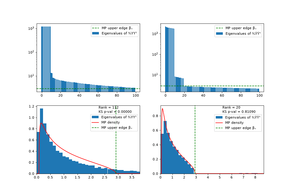
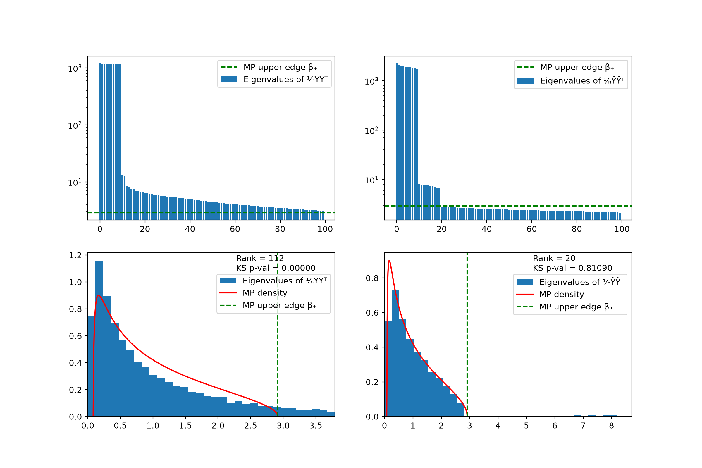
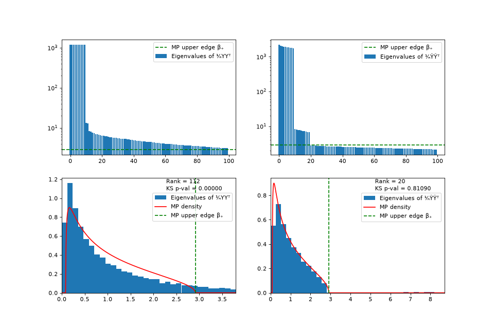
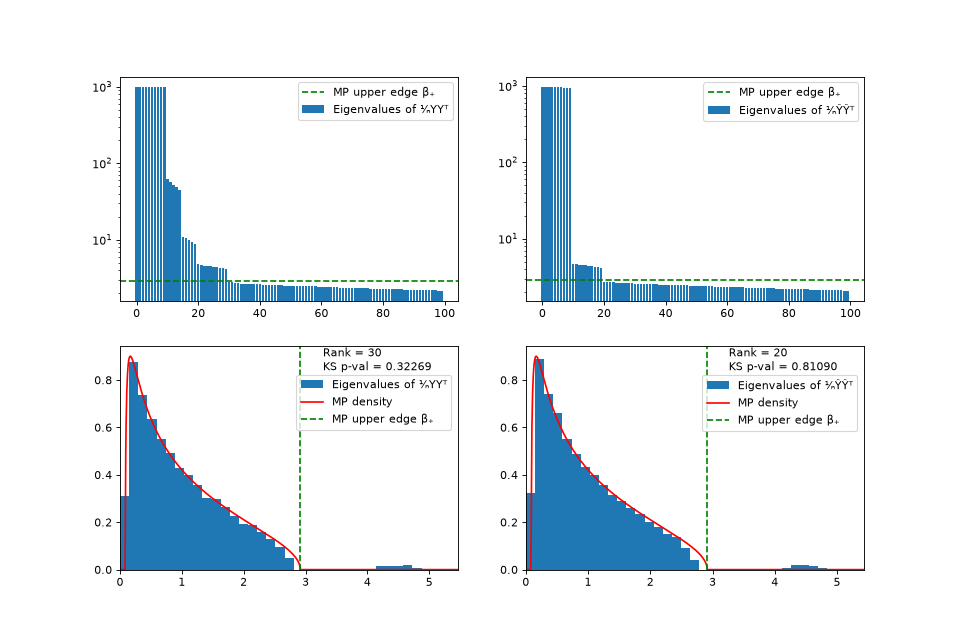
Spectrum of the data before (left) and after (right) applying the normalization of BRINE.

We observe that the eigenvalue spectrum of the normalized ¹⁄ₙŶŶᵀ matrix follows the theoretical Marchenko-Pastur (MP) distribution and that the MP upper edge β₊ correctly matches the rank of the signal. On the other hand, the eigenvalue spectrum of ¹⁄ₙYYᵀ contains extra eigenvalues due to the abnormal noise and the threshold β₊ would identify more than 20 significant components.

Heteroskedastic noise with a block variance profile

In this example we apply BRINE on data with a 2x2 block heteroskedastic noise-variance profile, plus a few scattered high-variance rows and columns — the simulation setup used in Figure 1 of the BRINE paper.

The signal X consists of 10 strong and 10 weak components to which this heteroskedastic noise was added to create the data matrix Y.

Next, we run BRINE and plot the eigenvalue distributions by

1. Initializing the BRINE class with the data Y and calling run()

2. Calling the plot_mp_eigenvalues_and_densities function. The option show_only_significant=1 was specified to limit the x-axis to the first non-noise eigenvalue, since the largest signal eigenvalues are large.

import matplotlib.pyplot as plt
import numpy as np
from brine.brine import BRINE
from brine.examples import generate_Y_with_block_variance_profile

Y = generate_Y_with_block_variance_profile()
brine = BRINE(Y).run()
brine.plot_mp_eigenvalues_and_densities(show_only_significant=1)

(Source code, png, hires.png, pdf)

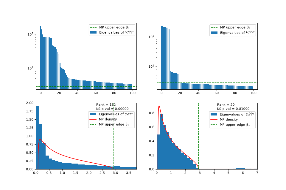
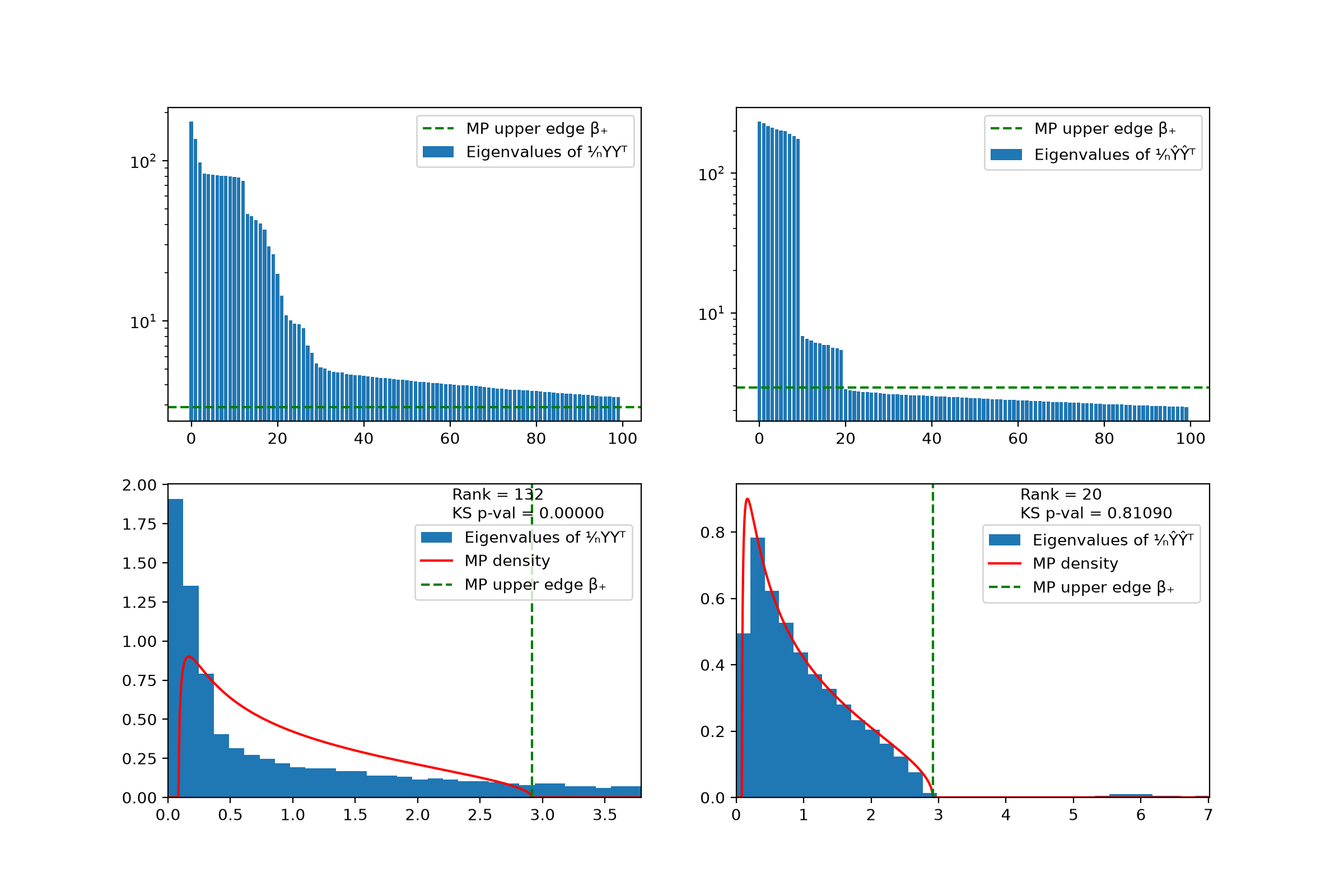
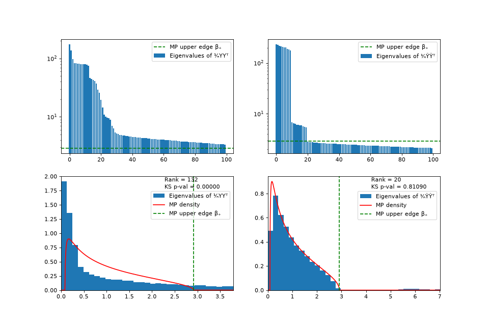
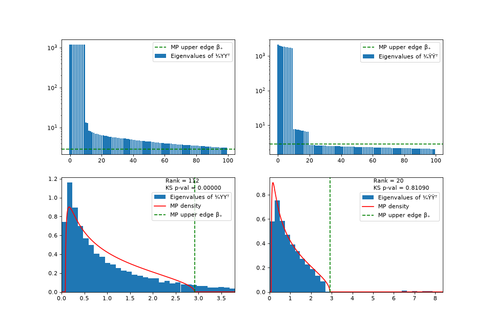
Spectrum of the data before (left) and after (right) applying the normalization of BRINE.

We observe that the eigenvalue spectrum of the normalized ¹⁄ₙŶŶᵀ matrix follows the theoretical Marchenko-Pastur (MP) distribution and that the MP upper edge β₊ correctly matches the rank of the signal. On the other hand, the eigenvalue spectrum of ¹⁄ₙYYᵀ contains extra eigenvalues due to the high-variance rows and columns, well beyond the true rank of the signal.

DysonEqualizer examples

We generally recommend using BRINE (see above) for equalizing heteroskedastic noise. The original, non-iterative DysonEqualizer remains available below, e.g. for one-shot use or for comparison against BRINE.

Almost homoskedastic noise

In this example we apply the Dyson Equalizer on data with Gaussian almost homoskedastic noise.

The signal X consists of 10 strong and 10 weak components to which Gaussian noise was added to create the data matrix Y = X + E. The noise E was homoskedastic everywhere with the exception of 5 rows and 5 columns, which have abnormally strong noise.

1. Initializing the DysonEqualizer class with the data class Y and calling compute()

2. Calling the plot_mp_eigenvalues_and_densities function. The option show_only_significant=1 was specified to limit the x-axis to the first non-noise eigenvalue, since the larges signal eigenvalues are large.

import matplotlib.pyplot as plt
import numpy as np
from brine.dyson_equalizer import DysonEqualizer
from brine.examples import generate_Y_with_almost_homoskedastic_noise

Y = generate_Y_with_almost_homoskedastic_noise()
de = DysonEqualizer(Y).compute()
de.plot_mp_eigenvalues_and_densities(show_only_significant=1)

(Source code, png, hires.png, pdf)

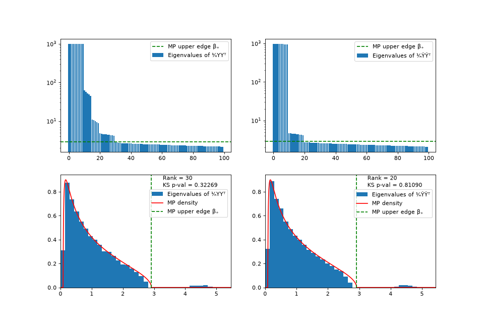
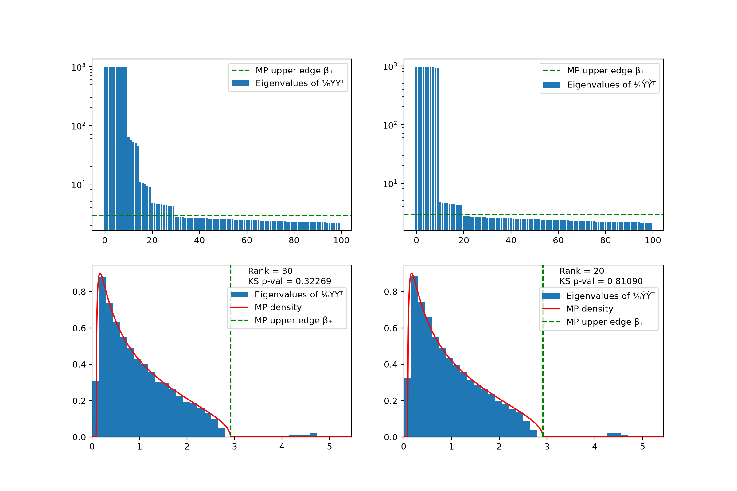
Spectrum of the data before (left) and after (right) applying the normalization of Dyson Equalizer.

We observe that the eigenvalue spectrum of the normalized ¹⁄ₙŶŶᵀ matrix follows the theoretical Marchenko-Pastur (MP) distribution and that the MP upper edge β₊ correctly matches the rank of the signal. On the other hand, the eigenvalue spectrum of ¹⁄ₙYYᵀ contains extra eigenvalues due to the abnormal noise and the threshold β₊ would identify more than 20 significant components.

Heteroskedastic noise

In this example we apply the Dyson Equalizer on data with Gaussian heteroskedastic noise. The signal X consists of 10 strong and 10 weak components to which Gaussian heteroskedastic noise was added to create the data matrix Y.

Next, we compute the Dyson Equalizer and plot the eigenvalues distributions by

1. Initializing the DysonEqualizer class with the data class Y and calling compute()

2. Calling the plot_mp_eigenvalues_and_densities function. The option show_only_significant=1 was specified to limit the x-axis to the first non-noise eigenvalue, since the larges signal eigenvalues are large.

import matplotlib.pyplot as plt
import numpy as np
from brine.dyson_equalizer import DysonEqualizer
from brine.examples import generate_Y_with_heteroskedastic_noise

Y = generate_Y_with_heteroskedastic_noise()
de = DysonEqualizer(Y).compute()
de.plot_mp_eigenvalues_and_densities(show_only_significant=1)

(Source code, png, hires.png, pdf)

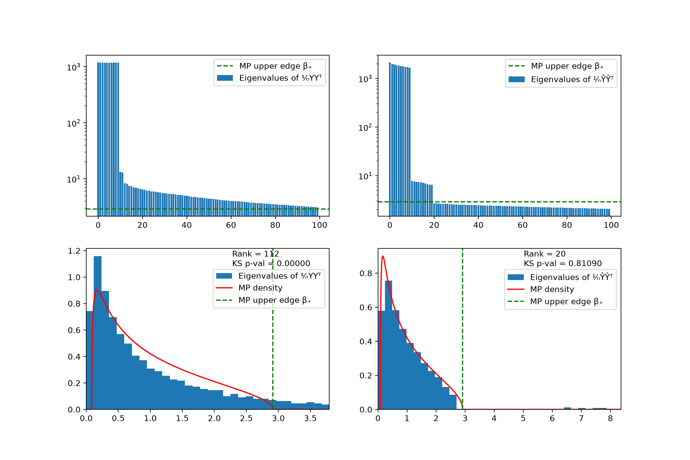
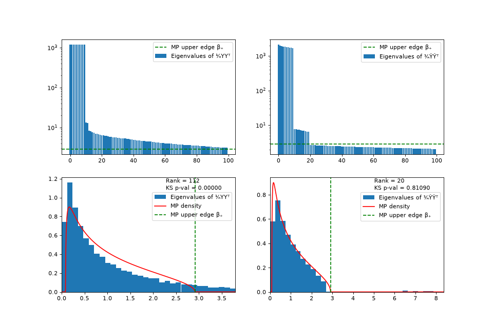
Spectrum of the data before (left) and after (right) applying the normalization of Dyson Equalizer.

We observe that the eigenvalue spectrum of the normalized ¹⁄ₙŶŶᵀ matrix follows the theoretical Marchenko-Pastur (MP) distribution and that the MP upper edge β₊ correctly matches the rank of the signal.