brine.plots module

The brine.plots module provides functions to create useful plots

brine.plots.plot_mp_cdf(eigs: ndarray, gamma: float, sigma: float | None = 1, show_only_significant_right_margin: float = 0.3, matrix_label: str = 'X', ax: Axes | None = None) → None

Plots the cdf of eigenvalues of the covariance matrix and compares to the Marchenko-Pastur distribution

This function assumes the input are the eigenvalues of a covariance matrix of a random matrix whose entries have variance 1. These eigenvalues follow the Marchenko-Pastur distribution.

Parameters:

eigs: (n) numpy.array

The array of eigenvalues (e.g. of a covariance matrix) to plot

gamma: float

The ratio between the dimensions of the matrix (between 0 and 1)

sigma: float, optional

The standard deviation of the random variable. If not specified it will be inferred so that the median matches the theoretical KS distribution

show_only_significant_right_margin: float, optional

Specifies the size of the right margin (defaults to 0.3) from the largest eigenvalue selected by the show_only_significant option

matrix_label: str, optional

The name of the matrix that will be used as label (defaults to X)

ax: plt.Axes, optional

A matplotlib Axes object. If none is provided, a new figure is created.

See also

brine.algorithm.marchenko_pastur_cdf

brine.plots.plot_mp_density(eigs: ndarray, gamma: float, sigma: float | None = None, show_only_significant: int = None, show_only_significant_right_margin: float = 0.3, matrix_label: str = 'X', bins: int | str | Sequence = 'sqrt', ax: Axes | None = None) → None

Plots the density of eigenvalues of the covariance matrix and compares to the Marchenko-Pastur distribution

This function assumes the input are the eigenvalues of a covariance matrix of a random matrix whose entries have variance 1. These eigenvalues follow the Marchenko-Pastur distribution.

Parameters:

eigs: (n) numpy.array

The array of eigenvalues (e.g. of a covariance matrix) to plot

gamma: float

The ratio between the dimensions of the matrix (between 0 and 1)

sigma: float, optional

The standard deviation of the random variable. If not specified it will be inferred so that the median matches the theoretical KS distribution

show_only_significant: int, optional

Set this value to show only a small number of significant eigenvalues (defaults to None) This option is useful is some of the signal eigenvalues are much bigger than the noise. Set to zero to show only significant eigenvalues within the margin indicated by show_only_significant_right_margin

show_only_significant_right_margin: float, optional

Specifies the size of the right margin (defaults to 0.3) from the largest eigenvalue selected by the show_only_significant option

matrix_label: str, optional

The name of the matrix that will be used as label (defaults to X)

bins: int or sequence or str, default: ‘sqrt’

The bins parameter used to build the histogram.

ax: plt.Axes, optional

A matplotlib Axes object. If none is provided, a new figure is created.

See also

brine.algorithm.marchenko_pastur

matplotlib.pyplot.Axes.hist

Examples

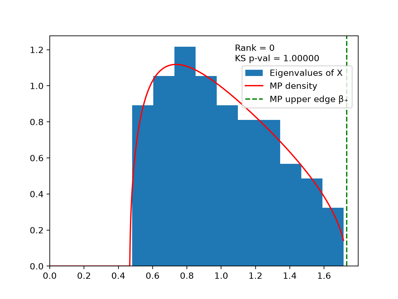
We generate a random matrix X of size (100, 1000) and show that the eigenvalues of the covariance matrix Y = ¹⁄ₙXXᵀ follow a Marchenko-Pastur distribution.

import numpy as np
from brine.plots import plot_mp_density

m, n = 100, 1000
X = np.random.normal(size=(m, n))
Y = X @ X.T / n
eigs = sorted(np.linalg.eigvals(Y), reverse=True)

plot_mp_density(eigs, gamma=m/n)

(Source code, png, hires.png, pdf)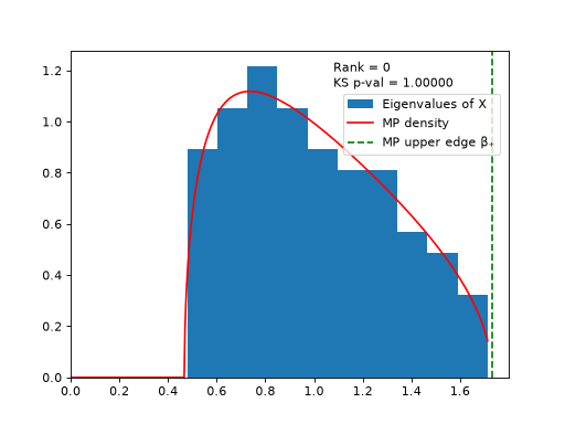

Eigenvalues plot of a random matrix

brine.plots.plot_mp_density_convergence(eigs_list: list[ndarray], gamma: float, show_only_significant: int = None, show_only_significant_right_margin: float = 0.3, matrix_labels: list[str] = None, cmap: str = 'cividis', bins: int | str | Sequence = 'sqrt', ax: Axes | None = None) → None

Plots the density of eigenvalues of a series of covariance matrices and compares them to the Marchenko-Pastur distribution

This function assumes the input are the eigenvalues of a covariance matrix of a random matrix whose entries have variance 1. These eigenvalues follow the Marchenko-Pastur distribution.

Parameters:

eigs_list: (n) numpy.array

A list of arrays of eigenvalues (e.g. of a series of covariance matrices) to plot

gamma: float

The ratio between the dimensions of the matrix (between 0 and 1)

show_only_significant: int, optional

Set this value to show only a small number of significant eigenvalues (defaults to None) This option is useful is some of the signal eigenvalues are much bigger than the noise. Set to zero to show only significant eigenvalues within the margin indicated by show_only_significant_right_margin

show_only_significant_right_margin: float, optional

Specifies the size of the right margin (defaults to 0.3) from the largest eigenvalue selected by the show_only_significant option

matrix_labels: list[str], optional

The labels for each eigenvalue in the list. If not provided, numbers from 0 to n-1 will be used

cmap: str, optional

The matplotlib colormap to use for the density plot

bins: int or sequence or str, default: ‘sqrt’

The bins parameter used to build the histogram.

ax: plt.Axes, optional

A matplotlib Axes object. If none is provided, a new figure is created.

See also

brine.algorithm.marchenko_pastur

matplotlib.pyplot.Axes.hist

Examples

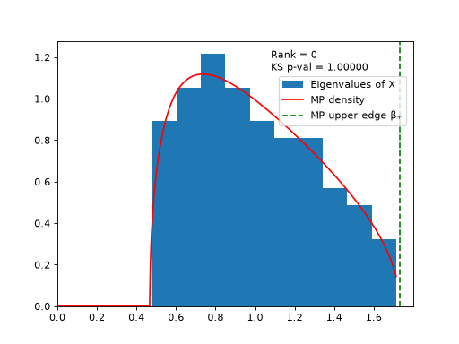
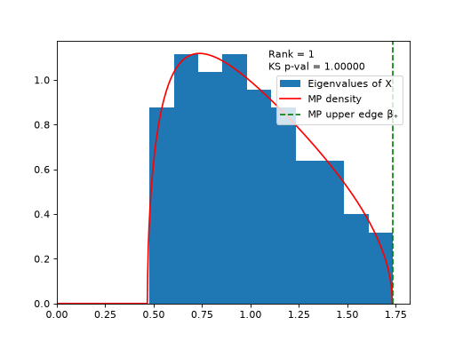
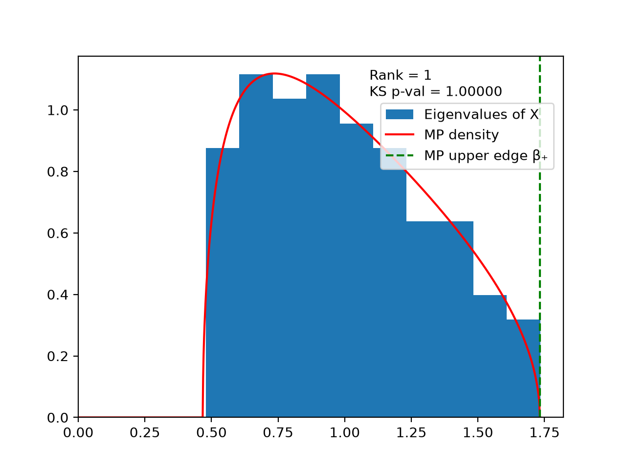
We generate a random matrix X of size (100, 1000) and show that the eigenvalues of the covariance matrix Y = ¹⁄ₙXXᵀ follow a Marchenko-Pastur distribution.

import numpy as np
from brine.plots import plot_mp_density

m, n = 100, 1000
X = np.random.normal(size=(m, n))
Y = X @ X.T / n
eigs = sorted(np.linalg.eigvals(Y), reverse=True)

plot_mp_density(eigs, gamma=m/n)

(Source code, png, hires.png, pdf)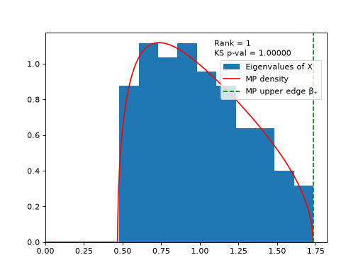

Eigenvalues plot of a random matrix

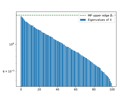
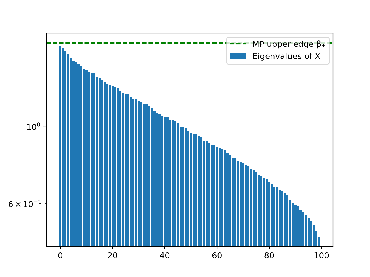
brine.plots.plot_mp_eigenvalues(eigs: ndarray, gamma: float, eigenvalues_to_show: int = 100, sigma: float | None = None, log_y: bool = True, matrix_label: str = 'X', ax: Axes | None = None) → None

Plots the eigenvalues of the covariance matrix and compares to the Marchenko-Pastur threshold

This function assumes the input are the eigenvalues of a covariance matrix of a random matrix whose entries have variance 1. These eigenvalues follow the Marchenko-Pastur distribution.

Parameters:

eigs: (n) numpy.array

The array of eigenvalues (e.g. of a covariance matrix) to plot

gamma: float

The ratio between the dimensions of the matrix (between 0 and 1)

sigma: float, optional

The standard deviation of the random variable. If not specified it will be inferred so that the median matches the theoretical KS distribution

eigenvalues_to_show: int, optional

The number of eigenvalues to show in the plot (defaults to 100)

log_y: bool, optional

Whether the y-axis should be logarithmic (defaults to True)

matrix_label: str, optional

The name of the matrix that will be used as label (defaults to X)

ax: plt.Axes, optional

A matplotlib Axes object. If none is provided, a new figure is created.

See also

brine.algorithm.marchenko_pastur

Examples

We generate a random matrix X of size (100, 1000) and show that the eigenvalues of the covariance matrix Y = ¹⁄ₙXXᵀ follow a Marchenko-Pastur distribution.

import numpy as np
from brine.plots import plot_mp_eigenvalues

m, n = 100, 1000
X = np.random.normal(size=(m, n))
Y = X @ X.T / n
eigs = sorted(np.linalg.eigvals(Y), reverse=True)

plot_mp_eigenvalues(eigs, gamma=m/n)

(Source code, png, hires.png, pdf)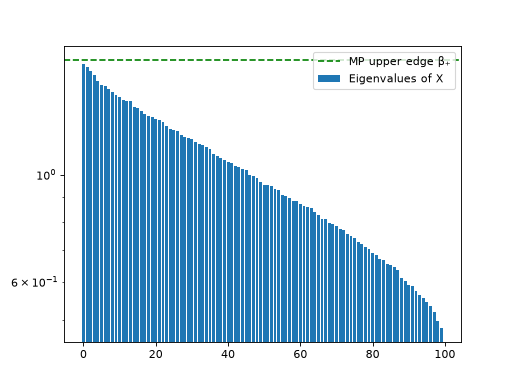

Eigenvalues plot of a random matrix