Find the Elbow Point Using the Kneedle Algorithm

Automatically selects the effective dimensionality from a decreasing eigenvalue sequence. The algorithm log-transforms the eigenvalues, normalizes both axes to the unit interval, draws a straight line between the first and last points, and returns the index of the point with the greatest perpendicular distance from that line. This point corresponds to the "elbow" where the eigenvalue decay transitions from steep to flat.

Usage

find_elbow_kneedle(eigenvalues)

Arguments

eigenvalues

Numeric vector of eigenvalues, typically in decreasing order. Non-positive values are automatically replaced with the preceding value to ensure a valid log transform. Must have length >= 3 for a meaningful result; if shorter, the full length is returned.

Value

An integer: the 1-based index of the elbow point. For example, a return value of 5 means the first 5 eigenvalues capture the dominant signal.

Details

MOSAIC calls this function internally at two stages: (1) to choose the per-sample rank from each coupling matrix eigendecomposition, and (2) to choose the global rank from the aggregated projection.

See also

plot_eigen for visualizing eigenvalue spectra.

Examples

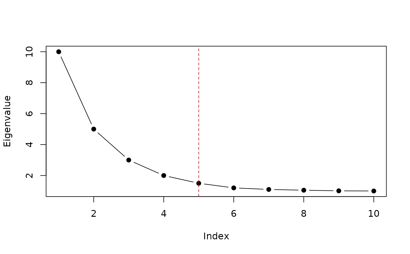
# Typical eigenvalue decay with a clear elbow at position 3
eigenvalues <- c(10, 5, 3, 2, 1.5, 1.2, 1.1, 1.05, 1.01, 1.0)
find_elbow_kneedle(eigenvalues)
#> [1] 5
# Returns 3

# Visualize the elbow
plot(eigenvalues, type = "b", pch = 19, xlab = "Index", ylab = "Eigenvalue")
abline(v = find_elbow_kneedle(eigenvalues), col = "red", lty = 2)