Application: Cross-sample Comparison
Ruiqi Li
08/20/2024
Source:vignettes/LMD_cross_comparison_demo.Rmd
LMD_cross_comparison_demo.RmdLoading Data
One of the downstream tasks for LMD is cross-sample comparison to identify sample-enriched or shared cell populations without the need for integration and differential abundance testing. Here we use a 10x mouse embryonic skin dataset. The preprocessed Seurat object for this tutorial can be downloaded from figshare for Mutant and figshare for Wildtype.
##### Load required R libraries
library("LocalizedMarkerDetector")
library("ggplot2")
library("Seurat")
library("SeuratWrappers")
library("patchwork")
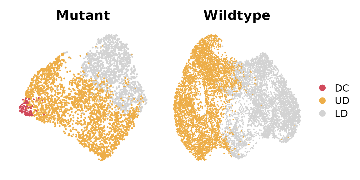
This dataset includes a SmoM2 mutant sample with a paired wildtype sample, both collected at embryonic day 13.5. We can visualize these two samples using UMAP, with cells color-coded by cell types.
##### Load Data
dir.path0 = "~/" # Specify the directory path where the data is saved
file_name1 = "data_S_smom2_dermal_E13.5_MUT.rds" # Specify the file name for saving the mutant
file_name2 = "data_S_smom2_dermal_E13.5_CTL.rds" # Specify the file name for saving the wildtype
data_S_MUT <- readRDS(file.path(dir.path0,file_name1))
data_S_CTL <- readRDS(file.path(dir.path0,file_name2))

p1 = DimPlot(data_S_MUT,
          group.by = "celltype", shuffle = TRUE, cols = c("DC"="#d1495b", "UD" = "#edae49", "LD" = "#d3d3d3")) + ggtitle("Mutant") & NoAxes()
p2 = DimPlot(data_S_CTL,
          group.by = "celltype", shuffle = TRUE, cols = c("DC"="#d1495b", "UD" = "#edae49", "LD" = "#d3d3d3")) + ggtitle("Wildtype") & NoAxes()
p1 + p2 + plot_layout(guides = "collect")
Running LMD and Identifying localized gene modules
Next, we run LMD and identify gene modules on the mutant sample.
#### Prepare data
dat = as.matrix(data_S_MUT[["RNA"]]@data)
# Keep genes express > 10 cells and less than 50% of cells
Gene_detected_count <- apply(dat > apply(dat,2,median),1,sum)
selected_genes = names(Gene_detected_count)[(Gene_detected_count >= 10) & (Gene_detected_count <= ncol(dat) * 0.5)]
dat = dat[selected_genes,,drop = FALSE]
# Extract top 14 PCs (# of PC based on Elbow Plot)
feature_space = Embeddings(data_S_MUT[["pca"]])[,1:FindPC(data_S_MUT)]
##### RunLMD
lmd_score_res = LMD(dat, feature_space, max_time = 2^20)
#> Constructing KNN graph
#> Remove 0 genes which express in less than 5 cells
#> Calculate LMD score profile for large data...
#> Run doubly stochastic on affinity matrix...
#>
#> max diffusion time:2^ 10

res = show_result_lmd(lmd_score_res)
##### Identify Gene Modules
if(!"alra" %in% names(data_S_MUT@assays)){
  data_S_MUT <- RunALRA(data_S_MUT, assay = "RNA")
  DefaultAssay(data_S_MUT) <- "RNA"
}
dat_alra = as.matrix(data_S_MUT[["alra"]]@data)[names(res$cut_off_gene),]
dist = CalculateGeneDistance(dat_alra, method = "jaccard")

gene_partition = ClusterGenes(dist, clustering_method = "average", deepSplit = 2)
#>  ..cutHeight not given, setting it to 0.986  ===>  99% of the (truncated) height range in dendro.
#>  ..done.
#> Filtering out outlier genes in each module:  478  genes left.
levels(gene_partition) = 1:nlevels(gene_partition)
table(gene_partition)
#> gene_partition
#>  1  2  3  4  5  6  7  8  9 10 11 12 13 14 15 16 17 18 19 20
#> 24 16 65 18 10 16 12 26 19 16 39 15 37 40 16 26 21 29 11 22
Computing module activity scores for both mutant and wildtype samples
Next, we calculate the module activity score for each module in both the mutant and wildtype samples.
Note: This step is CPU-intensive and may take 4 to 5 minutes to complete.
data_S_MUT = AddModuleActivityScore(data_S_MUT, gene_partition = gene_partition)
#> Start Loop
data_S_CTL = AddModuleActivityScore(data_S_CTL, gene_partition = gene_partition)
#> Start Loop
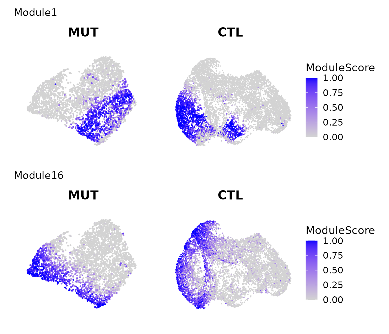
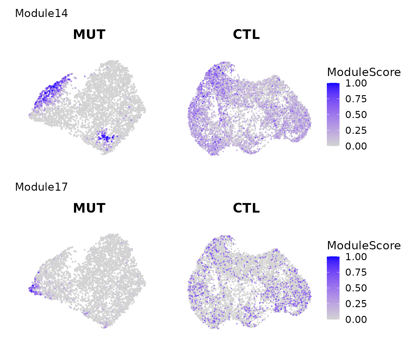
Then we can visualize the expression patterns of gene modules across both samples.
Modules reflecting functional similar cell populations between mutant and WT
Here we show two modules that are localized in both mutant and wildtype.
library(ggplotify)
pl = lapply(c("Module1","Module16"), function(module_name){
  pl = lapply(c("MUT","CTL"), function(i){
    FeaturePlot(get(paste0("data_S_",i)), features = c(module_name), order = TRUE) + scale_color_gradient(low = "lightgrey", high = "blue", limits = c(0,1)) + ggtitle(i) & labs(color = "ModuleScore") & NoAxes()
  })
  p = as.ggplot(wrap_plots(pl, nrow = 1) + plot_layout(guides = "collect") + plot_annotation(title = module_name))
})
p = wrap_plots(pl,ncol = 1)
p
Modules reflecting mutant-enriched cell populations
Here we show two modules that are only localized in mutant and dispersed in wildtype.
library(ggplotify)
pl = lapply(c("Module14","Module17"), function(module_name){
  pl = lapply(c("MUT","CTL"), function(i){
    FeaturePlot(get(paste0("data_S_",i)), features = c(module_name), order = TRUE) + scale_color_gradient(low = "lightgrey", high = "blue", limits = c(0,1)) + ggtitle(i) & labs(color = "ModuleScore") & NoAxes()
  })
  p = as.ggplot(wrap_plots(pl, nrow = 1) + plot_layout(guides = "collect") + plot_annotation(title = module_name))
})
p = wrap_plots(pl,ncol = 1)
p