LMD Tutorial

Overview

Localized Marker Detector (LMD) is a computational framework designed for the identification of gene expression markers localized to specific cell populations within single-cell RNA sequencing data. The major workflow of LMD comprises the following three main steps:

Step1. Constructing a cell-cell affinity graph
Step2. Diffusing the gene expression value across the cell graph
Step3. Assigning a score to each gene based on the dynamics of its diffusion process
Optional Downstream tasks
- Identifying gene modules and characterizing functional cell groups
- Cross-sample comparison

Loading required R packages

##### Load required R libraries
library("LocalizedMarkerDetector")
library("Seurat")
library("SeuratWrappers")
library("tictoc")
library("ggplot2")
library("patchwork")

Preparing input data

Loading example data

The preprocessed Seurat object for this tutorial can be downloaded from figshare. The preprocessing step can be refer to the Tabula Muris workflow(Consortium et al. 2018).

dir.path0 = "~/" # Specify the directory path where you want to save the data
file_name = "marrow_facs.rds" # Specify the file name for saving the data

if (!file.exists(file.path(dir.path0,file_name))) {
    options(timeout=6000)
    download.file("https://figshare.com/ndownloader/files/13092380", destfile = file.path(dir.path0,file_name), method = 'libcurl')
    # Check and upgrade the Seurat object if needed
    load(file.path(dir.path0,file_name))
    tiss <- UpdateSeuratObject(tiss)
    saveRDS(tiss, file = file.path(dir.path0,file_name))
}
tiss <- readRDS(file = file.path(dir.path0,file_name))

Extracting input data

Next, we prepare the following objects as input data from this Seurat object.

feature_space: A matrix containing the first 20 principal components (PCs) from PCA.
visual_space: A data frame containing the 2D t-SNE coordinates
dat: A matrix of log-normalized gene expression values, where rows correspond to genes and columns correspond to cells.
cell_label: Metadata related to the cells, such as cell type annotations, for visualization.

DefaultAssay(tiss) <- "RNA"
n_dim = dim(tiss@reductions$pca@cell.embeddings)[2]
feature_space = as.matrix(tiss@reductions$pca@cell.embeddings[,1:n_dim])
visual_space = data.frame(tiss@reductions$tsne@cell.embeddings)
dat = as.matrix(tiss[[DefaultAssay(tiss)]]@data)
cell_label = tiss$cell_ontology_class

Processing input data

We process the dat matrix by retaining only the genes that are detected in more than $10$ cells and less than $50\%$ of cells. A gene is considered “detected” in a cell if its expression level is greater than the median expression level of that cell.

Gene_detected_count <- apply(dat > apply(dat,2,median),1,sum)
selected_genes = (Gene_detected_count >= 10) & (Gene_detected_count <= ncol(dat) * 0.5)
dat = dat[selected_genes,,drop = FALSE]

Running LMD Step by Step

This provides a step-by-step tutorial for a better understanding of LMD. To directly obtain the output of LMD, skip to Running LMD in One Step.

Step1: Constructing a cell-cell affinity graph

We construct the cell-cell kNN graph (K= 5 in this example) using ConstructKnnGraph.

# Construct knn graph
knn_result = ConstructKnnGraph(knn = 5, feature_space = feature_space)
#> Constructing KNN graph
A = knn_result$adj_matrix # Adjacency Matrix
W = knn_result$graph # Symmetrized Graph ((A + AT) / 2)

# Plot knn graph
VisualizeGraph(affinity_m = W, label = cell_label, layout = visual_space) + 
  guides(color = guide_legend(ncol = 1, byrow = TRUE)) + 
  theme(
    legend.title = element_text(size = rel(0.7)),
    legend.text = element_text(size = rel(0.7)),
    legend.key.height = unit(1, "null"))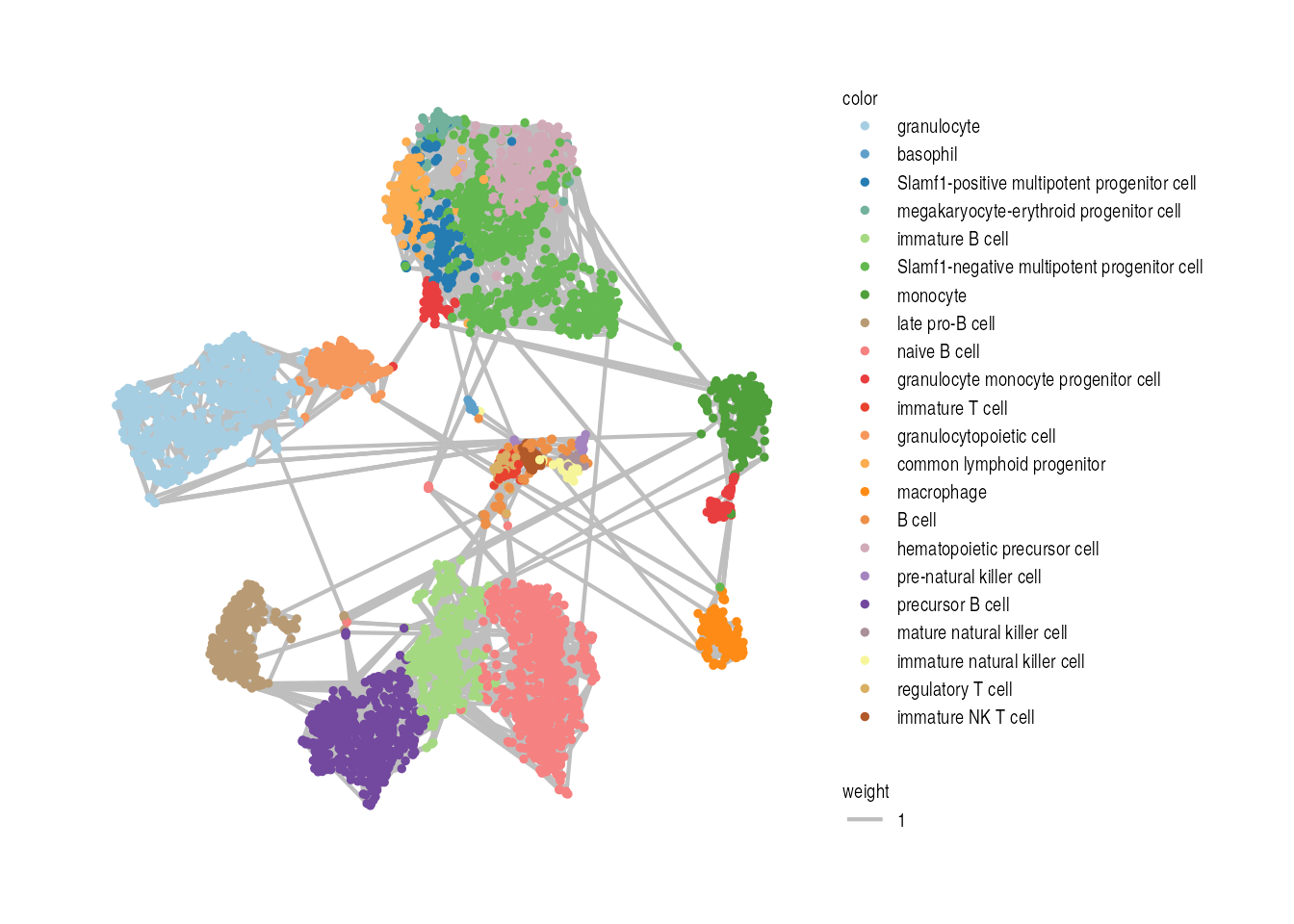

Step2: Diffusing the gene expression value across the cell graph

Next, we set the initial state of each gene by normalizing the expression matrix using RowwiseNormalize. We then construct a list of diffusion operators at different time scales using ConstructDiffusionOperators. By multiplying the initial state with the corresponding diffusion operators, we obtain the diffused state of each gene at the dyadic time scales $0,2^1,2^2,\dots$ . Finally, we can visualize the diffused state of each gene on the cell embedding.

# Construct a list of diffusion operators
P_ls = ConstructDiffusionOperators(W = W, max_time = 2^20)
#> Create a list of diffusion operators...
#>   |                                                                              |                                                                      |   0%  |                                                                              |=======                                                               |  10%  |                                                                              |=====================                                                 |  30%  |                                                                              |============================                                          |  40%  |                                                                              |===================================                                   |  50%  |                                                                              |==========================================                            |  60%  |                                                                              |=================================================                     |  70%  |                                                                              |========================================================              |  80%  |                                                                              |===============================================================       |  90%  |                                                                              |======================================================================| 100%
#> Converting diffusion operators to sparse matrices...
#> 
#> Max diffusion time: 16384
# Generate initial state for each gene
rho = RowwiseNormalize(dat[,colnames(W)])

Here we visualize the diffused state of Fcnb - a marker for granulocytopoietic cells, at four different time points: $t=0,t=2^1,t=2^4,$ and $t=2^{10}$ .

gene = "Fcnb"
VisualizeDiffusion(coord = visual_space,init_state = rho[gene,],P_ls = P_ls,check_time = c(0,2,2^4,2^10),gene_name = gene) & 
theme(
  plot.title = element_text(size = rel(0.7)),
  plot.subtitle = element_text(size = rel(0.7)),
  legend.title = element_text(size = rel(0.7)),
  legend.text = element_text(size = rel(0.7)) )

Step3: Obtain Diffusion KL score & LMD score

We measure the dynamics of the diffusion process for each gene using a score profile. This profile is calculated by the Kullback–Leibler (KL) divergence between the initial state and the diffused state, and then normalizing it by the KL divergence between the initial state and the equilibrium state.

We summarize this score profile into the LMD score, which is the cumulative sum of the score profile at all dyadic time steps. This LMD score can be used to rank the genes. Both the score profile and the LMD score are calculated using fast_get_lmds.

score_result = fast_get_lmds(W = W, init_state = rho, P_ls = P_ls, largeData = FALSE)

Now, we visualize three sets of genes expressing in different number of cells:

Expressed in approximately $20$ cells: Tlr11, 4933425H06Rik
Expressed in approximately $500$ cells: Fcnb, Uchl4
Expressed in approximately $2,500$ cells: Cd79a, Dock11

genes = c("Tlr11","Fcnb","Cd79a","4933425H06Rik","Uchl4","Dock11")
FeaturePlot(tiss, features = genes, ncol = 3, order = TRUE) & NoAxes() & theme(plot.title = element_text(size = rel(0.5)), legend.text = element_text(size = rel(0.5)))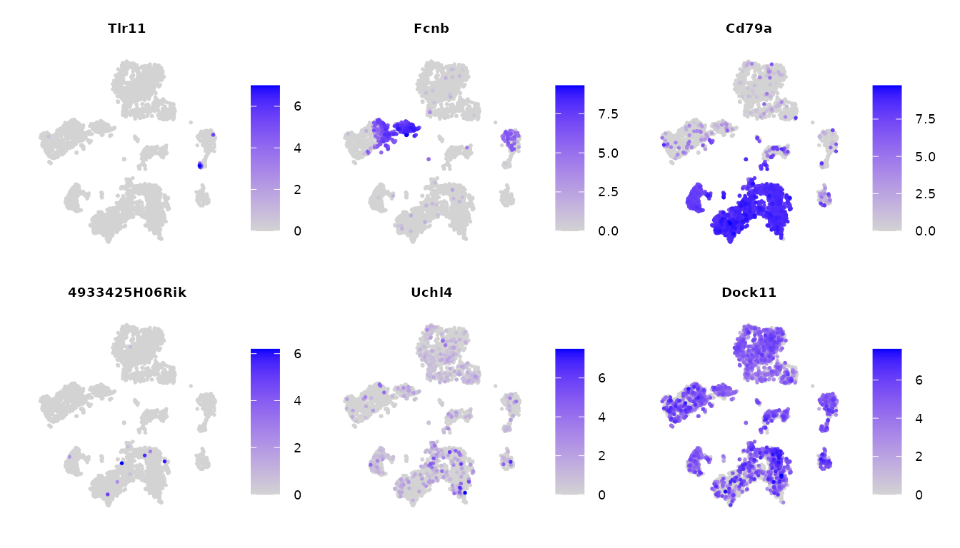

We visualize the score profiles for genes above. Genes with more localized patterns (Tlr11, Fcnb, Cd79a) tend to have smaller LMD scores (area under the curve) regardless of the number of cells in which they are expressed.

genes_label = rep(c("localized","non_localized"),each = 3)
VisualizeScorePattern(score_result$'score_profile', genes = genes, label_class = genes_label, facet_class = NULL, text = TRUE, normalize = TRUE) & theme(
    plot.title = element_text(size = rel(0.7)),
    plot.subtitle = element_text(size = rel(0.7)),
    axis.title.x = element_text(size = rel(0.7)), axis.title.y = element_text(size = rel(0.7)),
    axis.text.x = element_text(size = rel(0.7)), axis.text.y = element_text(size = rel(0.7)),
    legend.title = element_text(size = rel(0.7)),
    legend.text = element_text(size = rel(0.7)) )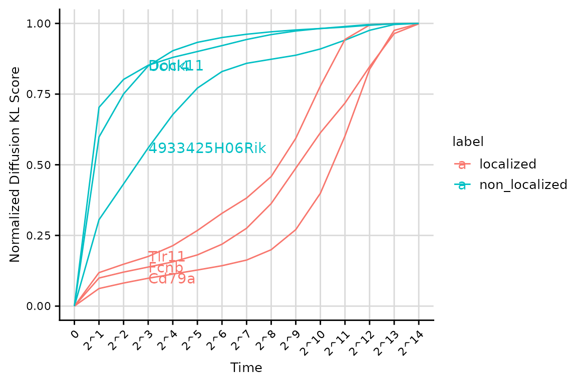

The results of the LMD can be presented in a table, displaying the LMD score and the rank for each gene.

res = show_result_lmd(score_result)
head(res$gene_table,10)
#>                  score rank
#> Mmp9          4.508234    1
#> 1100001G20Rik 4.624757    2
#> Itgb2l        4.627945    3
#> Lrg1          4.654115    4
#> C5ar1         4.737228    5
#> Retnlg        4.799311    6
#> Hp            4.799382    7
#> 1810033B17Rik 4.813253    8
#> Lcn2          4.825797    9
#> Chi3l1        4.828846   10

Running LMD in one step

LMD can be run in one step. In this case, the input is:

dat: the log-normalized gene expression data, where rows correspond to genes and columns correspond to cells.
feature_space: the first 20 principal components (PCs) of the dat.
knn: $k$ of the cell-cell kNN graph.

This example dataset contains 5,037 cells, running LMD should take 1 to 3 minutes to finish.

Note: The actual runtime can vary depending on your system’s matrix operation performance. To potentially reduce runtime and enhance performance, ensure that your R environment is configured with optimized BLAS/LAPACK libraries, such as OpenBLAS, which support parallel processing. For details on the specific setup used in this tutorial, please refer to Session information.

For more information on installing and configuring these libraries, visit OpenBLAS and R Administration and Installation.

# Load packages
library(LocalizedMarkerDetector)
library(tictoc)

tic()
score_result = LMD(dat, feature_space, knn = 5)
#> Constructing KNN graph
#> Remove 0 genes which express in less than 5 cells
#> Calculate LMD score profile for large data...
#> Run doubly stochastic on affinity matrix...
#> 
#> max diffusion time:2^ 14
toc()
#> 169.99 sec elapsed

Present the results of LMD in a table: the LMD score and the rank for each gene.

res = show_result_lmd(score_result)
head(res$gene_table,10)
#>                  score rank
#> Mmp9          4.508234    1
#> 1100001G20Rik 4.624757    2
#> Itgb2l        4.627945    3
#> Lrg1          4.654115    4
#> C5ar1         4.737228    5
#> Retnlg        4.799311    6
#> Hp            4.799382    7
#> 1810033B17Rik 4.813253    8
#> Lcn2          4.825797    9
#> Chi3l1        4.828846   10

Identifying Gene Modules

First, we select the top localized genes based on the knee point of the LMDS distribution.

res = show_result_lmd(score_result, kneeplot = TRUE)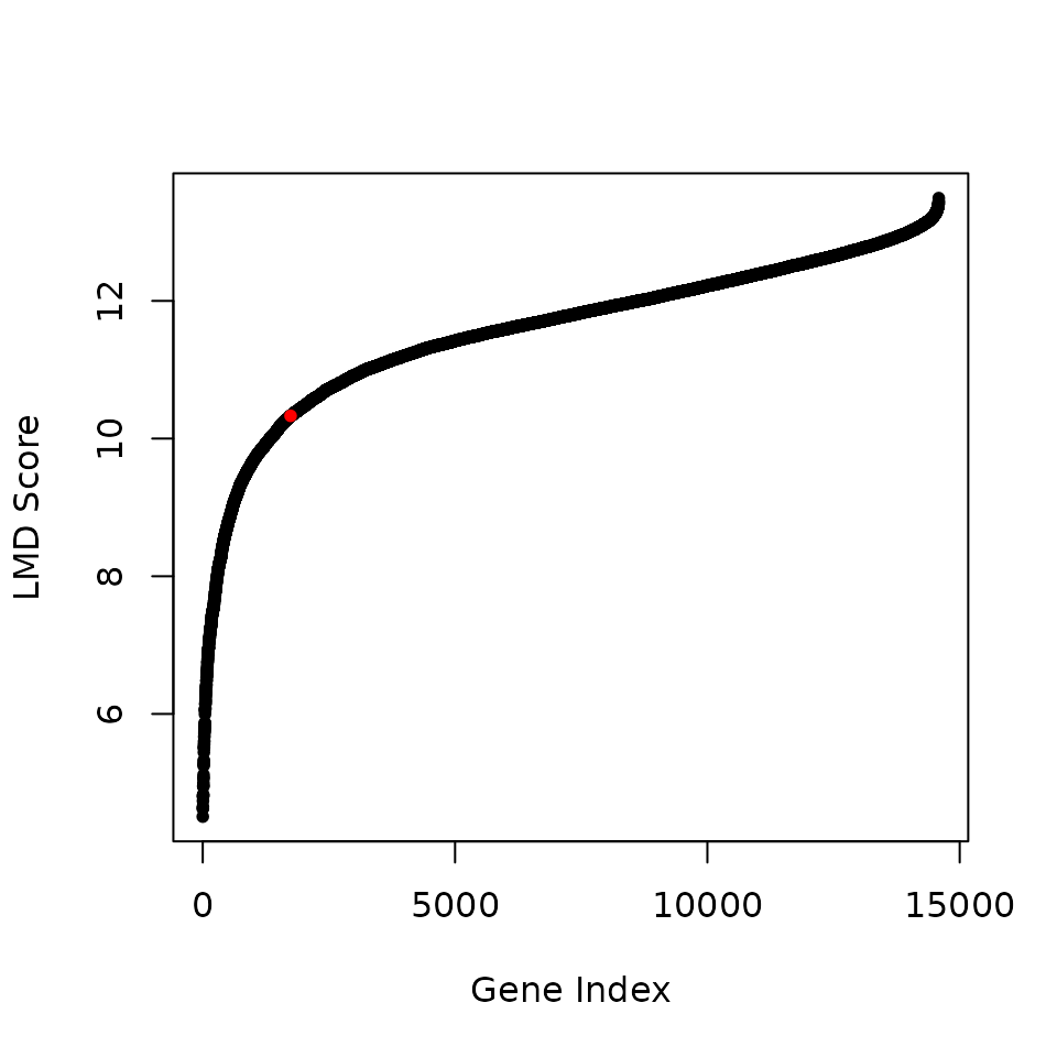

#> knee_point:  1741
top_lmd_genes = names(res$cut_off_gene)

Next, we compute the gene-gene pairwise Jaccard distance based on their expression levels over all cells using CalculateGeneDistance. We recommend users to apply ALRA imputation(Linderman et al. 2022) first to reduce the effect of drop-out events on the gene distance calculations.

Notes:

ALRA may produce different results with each run, leading to slight variations in the gene-gene distance and gene clustering results For reproducibility with this tutorial, users can download our preprocessed Seurat object, which includes the ALRA assay.
This step is time-consuming and may take 4 to 5 minutes to complete.

# tic()
# ALRA imputation
if(!"alra" %in% names(tiss@assays)){
  tiss <- RunALRA(tiss, assay = "RNA")
  DefaultAssay(tiss) <- "RNA"
}
dat_alra = as.matrix(tiss[["alra"]]@data)[top_lmd_genes,]

# Compute the gene-gene pairwise distance
dist = CalculateGeneDistance(dat_alra, method = "jaccard")
# toc()

After obtaining the gene-gene distance matrix dist, we cluster the genes using stats::hclust with average option and determine the gene modules using dynamicTreeCut::cutreeDynamic. Optionally, we remove outlier genes in each module with SML algorithm(Parisi et al. 2014) and discard modules containing fewer than 10 genes. All of these steps are performed using ClusterGenes.

gene_cl_res = ClusterGenes(dist, clustering_method = "average", return_tree = TRUE, deepSplit = 1)
#>  ..cutHeight not given, setting it to 0.976  ===>  99% of the (truncated) height range in dendro.
#>  ..done.
#> Filtering out outlier genes in each module:  1684  genes left.

We can visualize the pairwise distance matrix of genes. The sidebar and side tree represent the partitioning of genes into gene modules.

VisualizeGeneHeatmap(dist, gene_partition = gene_cl_res$gene_partition, gene_hree = gene_cl_res$gene_hree)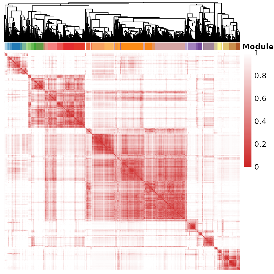

Computing Per-Cell Module Activity Scores

Next, we calculate the module activity score for each module using AddModuleActivityScore, which represents the probability of a module being expressed in a given cell. This score can be further used to visualize the expression patterns of each module and to identify the corresponding cells.

Note: This step is CPU-intensive and may take 4 to 5 minutes to complete. We also suggest considering alternative methods, such as Seurat::AddModuleScore, to visualize the gene module on cell embedding.

gene_partition = gene_cl_res$gene_partition
levels(gene_partition) = 1:nlevels(gene_partition) # rename gene modules

tiss = AddModuleActivityScore(tiss, gene_partition = gene_partition)

# Visualize patterns
(FeaturePlot(tiss, features = colnames(tiss@meta.data)[grepl("Module",colnames(tiss@meta.data))], order = TRUE, reduction = "tsne", ncol = 5) & NoAxes() & 
  scale_color_gradient(low = "lightgrey", high = "blue", limits = c(0,1)) & labs(color = "ModuleScore") & theme(
    plot.title = element_text(size = rel(0.5)),
    legend.title = element_text(size = rel(0.5)),
    legend.text = element_text(size = rel(0.5)) )) + plot_layout(guides = "collect")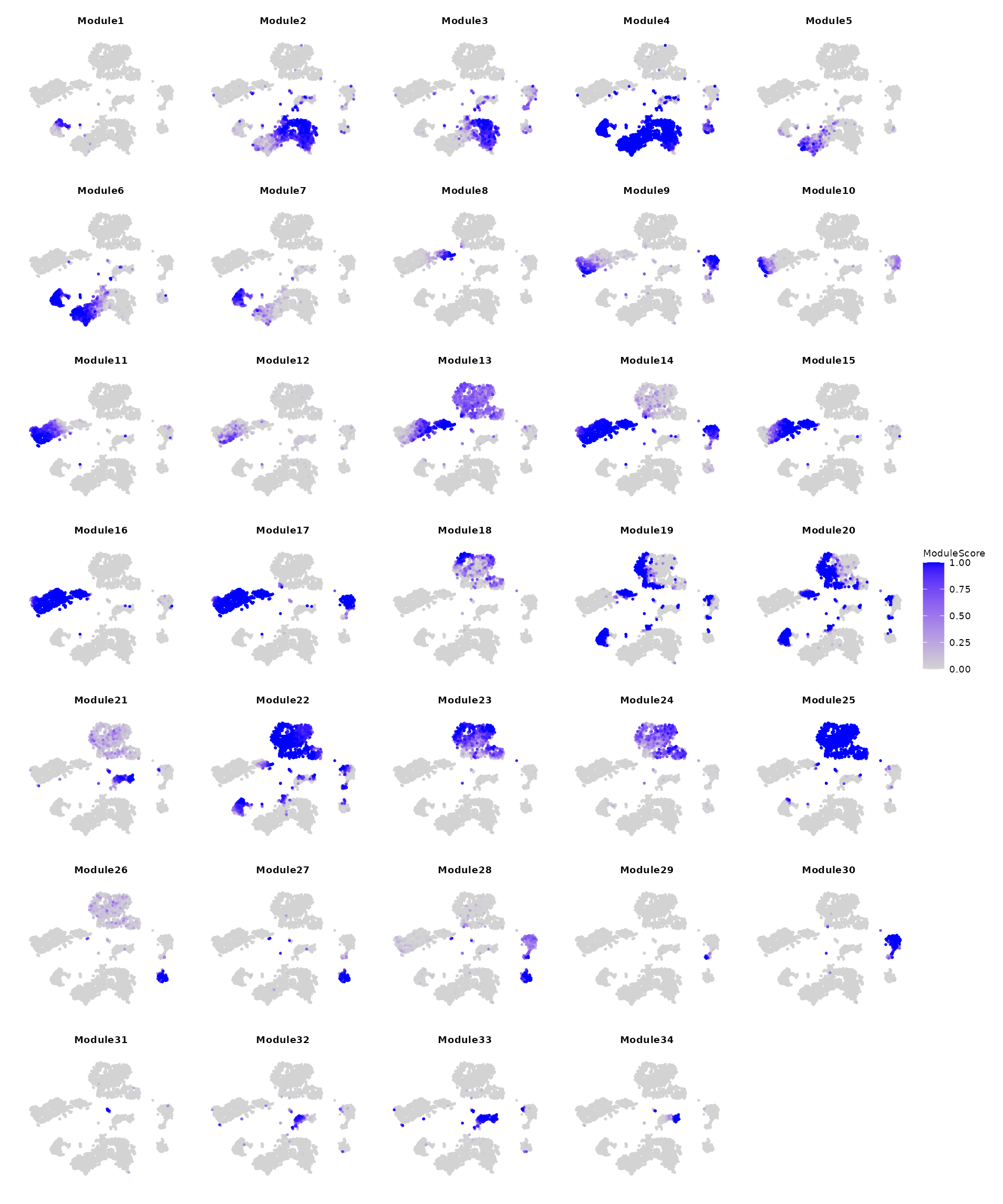

We can take a closer look at a module by examining several of its top localized genes.

module_id = 19
p1 = FeaturePlot(tiss, features = paste0("Module",module_id), order = TRUE, reduction = "tsne") + ggtitle(sprintf("Module%s (%d genes)",module_id,sum(gene_partition == module_id))) + labs(color = "ModuleScore") + NoAxes()
pl = FeaturePlot(tiss, features = names(gene_partition)[gene_partition == module_id][1:6],ncol = 3, order = TRUE) & NoAxes()
p = (p1 + pl + plot_layout(design = c("#BBB\nABBB\nABBB\n#BBB"))) & theme(
    plot.title = element_text(size = rel(0.5)),
    legend.title = element_text(size = rel(0.5)),
    legend.text = element_text(size = rel(0.5)) )
p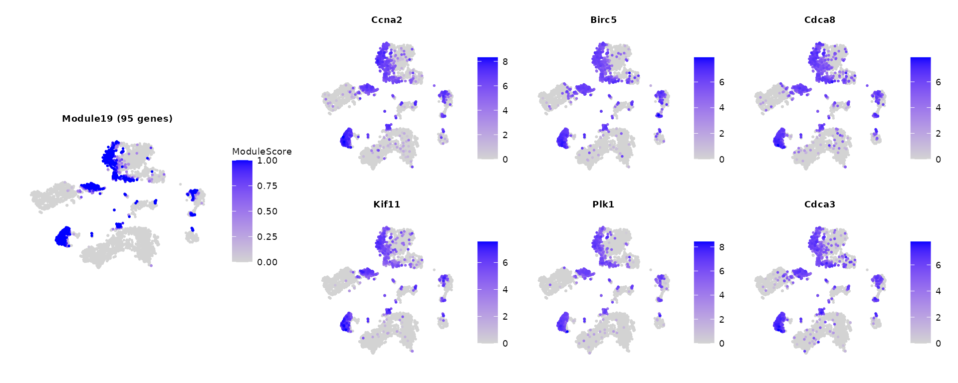

To better understand the biological functions of these gene modules, we can perform a series of functional enrichment analyses, such as Gene Ontology (GO) enrichment analysis(Wu et al. 2021) or Reactome Pathway Database enrichment analysis(Yu and He 2016). Here, we demonstrate the Reactome Pathway Database enrichment analysis using ReactomePA::enrichPathway for previous selected gene module, and we print its top 5 significantly enriched pathways.

library(ReactomePA)
library(org.Mm.eg.db)

bg_genes = rownames(dat) # Set all genes(after filtering) in the expression matrix as background genes
universe_df = data.frame("symbol" = bg_genes,"entrez" = mapIds(org.Mm.eg.db, keys=bg_genes, column="ENTREZID", keytype="SYMBOL"))
universe_df = universe_df[!is.na(universe_df$entrez),]
epathway_result <- enrichPathway(gene=universe_df[universe_df$symbol %in% names(gene_partition)[gene_partition == module_id],"entrez"],
                organism = "mouse",
                pAdjustMethod = "BH",
                pvalueCutoff = 0.05,
                universe = universe_df$entrez)

print(epathway_result@result[1:5,c('Description', 'GeneRatio', 'p.adjust')])
#>                          Description GeneRatio     p.adjust
#> R-MMU-1640170             Cell Cycle     30/47 3.388436e-23
#> R-MMU-69278      Cell Cycle, Mitotic     28/47 7.167466e-23
#> R-MMU-68886                  M Phase     21/47 6.462027e-17
#> R-MMU-68877     Mitotic Prometaphase     18/47 1.268621e-16
#> R-MMU-69620   Cell Cycle Checkpoints     18/47 1.228419e-15

Session information

sessionInfo()
#> R version 4.1.3 (2022-03-10)
#> Platform: x86_64-pc-linux-gnu (64-bit)
#> Running under: Ubuntu 20.04.4 LTS
#> 
#> Matrix products: default
#> BLAS:   /usr/lib/x86_64-linux-gnu/openblas-pthread/libblas.so.3
#> LAPACK: /usr/lib/x86_64-linux-gnu/openblas-pthread/liblapack.so.3
#> 
#> locale:
#>  [1] LC_CTYPE=en_US.UTF-8       LC_NUMERIC=C              
#>  [3] LC_TIME=en_US.UTF-8        LC_COLLATE=en_US.UTF-8    
#>  [5] LC_MONETARY=en_US.UTF-8    LC_MESSAGES=en_US.UTF-8   
#>  [7] LC_PAPER=en_US.UTF-8       LC_NAME=C                 
#>  [9] LC_ADDRESS=C               LC_TELEPHONE=C            
#> [11] LC_MEASUREMENT=en_US.UTF-8 LC_IDENTIFICATION=C       
#> 
#> attached base packages:
#> [1] stats4    stats     graphics  grDevices utils     datasets  methods  
#> [8] base     
#> 
#> other attached packages:
#>  [1] org.Mm.eg.db_3.14.0           AnnotationDbi_1.56.2         
#>  [3] IRanges_2.28.0                S4Vectors_0.32.4             
#>  [5] Biobase_2.54.0                BiocGenerics_0.40.0          
#>  [7] ReactomePA_1.38.0             patchwork_1.1.2              
#>  [9] ggplot2_3.3.6                 tictoc_1.2                   
#> [11] SeuratWrappers_0.3.1          SeuratObject_4.1.3           
#> [13] Seurat_4.3.0.1                LocalizedMarkerDetector_1.0.0
#> 
#> loaded via a namespace (and not attached):
#>   [1] utf8_1.2.2             spatstat.explore_3.2-1 reticulate_1.25       
#>   [4] R.utils_2.12.0         tidyselect_1.2.0       RSQLite_2.2.16        
#>   [7] htmlwidgets_1.5.4      grid_4.1.3             BiocParallel_1.28.3   
#>  [10] Rtsne_0.16             scatterpie_0.2.1       munsell_0.5.0         
#>  [13] codetools_0.2-18       ragg_1.3.2             ica_1.0-3             
#>  [16] future_1.27.0          miniUI_0.1.1.1         withr_2.5.0           
#>  [19] GOSemSim_2.20.0        spatstat.random_3.1-5  colorspace_2.0-3      
#>  [22] progressr_0.10.1       highr_0.11             knitr_1.48            
#>  [25] rstudioapi_0.14        ROCR_1.0-11            tensor_1.5            
#>  [28] DOSE_3.20.1            listenv_0.8.0          labeling_0.4.2        
#>  [31] GenomeInfoDbData_1.2.7 polyclip_1.10-0        bit64_4.0.5           
#>  [34] farver_2.1.1           pheatmap_1.0.12        treeio_1.18.1         
#>  [37] parallelly_1.32.1      vctrs_0.6.3            generics_0.1.3        
#>  [40] xfun_0.46              GenomeInfoDb_1.30.1    R6_2.5.1              
#>  [43] graphlayouts_1.0.0     rsvd_1.0.5             fgsea_1.20.0          
#>  [46] bitops_1.0-7           spatstat.utils_3.0-5   cachem_1.0.6          
#>  [49] gridGraphics_0.5-1     promises_1.2.0.1       scales_1.2.1          
#>  [52] enrichplot_1.14.2      ggraph_2.1.0           gtable_0.3.0          
#>  [55] globals_0.16.0         goftest_1.2-3          tidygraph_1.2.3       
#>  [58] rlang_1.1.1            systemfonts_1.1.0      splines_4.1.3         
#>  [61] lazyeval_0.2.2         checkmate_2.1.0        spatstat.geom_3.2-5   
#>  [64] BiocManager_1.30.18    yaml_2.3.10            reshape2_1.4.4        
#>  [67] abind_1.4-5            backports_1.4.1        httpuv_1.6.5          
#>  [70] qvalue_2.26.0          tools_4.1.3            ggplotify_0.1.2       
#>  [73] ellipsis_0.3.2         jquerylib_0.1.4        RColorBrewer_1.1-3    
#>  [76] dynamicTreeCut_1.63-1  ggridges_0.5.3         latex2exp_0.9.6       
#>  [79] Rcpp_1.0.9             plyr_1.8.7             zlibbioc_1.40.0       
#>  [82] progress_1.2.2         RCurl_1.98-1.8         purrr_1.0.2           
#>  [85] prettyunits_1.1.1      dbscan_1.1-12          deldir_1.0-6          
#>  [88] pbapply_1.5-0          viridis_0.6.2          cowplot_1.1.1         
#>  [91] zoo_1.8-10             ggrepel_0.9.1          cluster_2.1.2         
#>  [94] fs_1.6.4               magrittr_2.0.3         data.table_1.14.2     
#>  [97] RSpectra_0.16-1        scattermore_0.8        DO.db_2.9             
#> [100] reactome.db_1.77.0     lmtest_0.9-40          RANN_2.6.1            
#> [103] fitdistrplus_1.1-8     matrixStats_0.62.0     hms_1.1.2             
#> [106] mime_0.12              evaluate_0.24.0        xtable_1.8-4          
#> [109] gridExtra_2.3          compiler_4.1.3         tibble_3.2.1          
#> [112] shadowtext_0.1.2       KernSmooth_2.23-20     crayon_1.5.1          
#> [115] R.oo_1.25.0            htmltools_0.5.8.1      ggfun_0.1.3           
#> [118] later_1.3.0            aplot_0.2.1            tidyr_1.2.0           
#> [121] DBI_1.1.3              tweenr_2.0.2           rappdirs_0.3.3        
#> [124] MASS_7.3-55            Matrix_1.6-1           cli_3.6.1             
#> [127] R.methodsS3_1.8.2      parallel_4.1.3         igraph_1.3.4          
#> [130] pkgconfig_2.0.3        pkgdown_2.1.0          sp_1.5-0              
#> [133] philentropy_0.7.0      plotly_4.10.0          spatstat.sparse_3.0-2 
#> [136] ggtree_3.2.1           bslib_0.8.0            XVector_0.34.0        
#> [139] yulab.utils_0.0.9      stringr_1.4.1          digest_0.6.36         
#> [142] sctransform_0.3.5      RcppAnnoy_0.0.19       graph_1.72.0          
#> [145] Biostrings_2.62.0      spatstat.data_3.0-1    fastmatch_1.1-3       
#> [148] rmarkdown_2.27         leiden_0.4.2           tidytree_0.4.5        
#> [151] uwot_0.1.14            graphite_1.40.0        shiny_1.7.2           
#> [154] lifecycle_1.0.3        nlme_3.1-155           jsonlite_1.8.8        
#> [157] desc_1.4.3             viridisLite_0.4.1      fansi_1.0.3           
#> [160] pillar_1.9.0           lattice_0.20-45        GO.db_3.14.0          
#> [163] KEGGREST_1.34.0        fastmap_1.2.0          httr_1.4.4            
#> [166] survival_3.2-13        glue_1.6.2             remotes_2.4.2         
#> [169] FNN_1.1.3.1            png_0.1-7              bit_4.0.4             
#> [172] ggforce_0.4.1          stringi_1.7.8          sass_0.4.9            
#> [175] blob_1.2.3             textshaping_0.4.0      memoise_2.0.1         
#> [178] dplyr_1.1.3            ape_5.6-2              irlba_2.3.5           
#> [181] future.apply_1.9.0

References

Consortium, Tabula Muris, Overall coordination Schaum Nicholas 1 Karkanias Jim 2 Neff Norma F. 2 May Andrew P. 2 Quake Stephen R. quake@ stanford. edu 2 3 f Wyss-Coray Tony twc@ stanford. edu 4 5 6 g Darmanis Spyros spyros. darmanis@ czbiohub. org 2 h, Logistical coordination Batson Joshua 2 Botvinnik Olga 2 Chen Michelle B. 3 Chen Steven 2 Green Foad 2 Jones Robert C. 3 Maynard Ashley 2 Penland Lolita 2 Pisco Angela Oliveira 2 Sit Rene V. 2 Stanley Geoffrey M. 3 Webber James T. 2 Zanini Fabio 3, and Computational data analysis Batson Joshua 2 Botvinnik Olga 2 Castro Paola 2 Croote Derek 3 Darmanis Spyros 2 DeRisi Joseph L. 2 27 Karkanias Jim 2 Pisco Angela Oliveira 2 Stanley Geoffrey M. 3 Webber James T. 2 Zanini Fabio 3. 2018. “Single-Cell Transcriptomics of 20 Mouse Organs Creates a Tabula Muris.” Nature 562 (7727): 367–72.

Linderman, George C, Jun Zhao, Manolis Roulis, Piotr Bielecki, Richard A Flavell, Boaz Nadler, and Yuval Kluger. 2022. “Zero-Preserving Imputation of Single-Cell RNA-Seq Data.” Nature Communications 13 (1): 192.

Parisi, Fabio, Francesco Strino, Boaz Nadler, and Yuval Kluger. 2014. “Ranking and Combining Multiple Predictors Without Labeled Data.” Proceedings of the National Academy of Sciences 111 (4): 1253–58.

Wu, Tianzhi, Erqiang Hu, Shuangbin Xu, Meijun Chen, Pingfan Guo, Zehan Dai, Tingze Feng, et al. 2021. “clusterProfiler 4.0: A Universal Enrichment Tool for Interpreting Omics Data.” The Innovation 2 (3).

Yu, Guangchuang, and Qing-Yu He. 2016. “ReactomePA: An r/Bioconductor Package for Reactome Pathway Analysis and Visualization.” Molecular BioSystems 12 (2): 477–79.

Ruiqi Li, Francesco Strino, Rihao Qu

08/20/2024