DAseq Tutorial
tutorial.RmdDA-seq tutorial
Overview
This tutorial shows basic steps to run DAseq on scRNA-seq datasets.
Data used in this tutorial is from Sade-Feldman, Moshe, et al. (Cell. 2018). The goal is to compare immune cells from melanoma patients that respond or not respond to immune checkpoint therapy: responders (R) and non-responders (NR), and identify cell subpopulations with differential abundance (DA) between them.
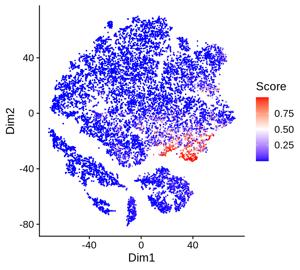
With DAseq, five DA cell subpopulations are detected and characterized.
library(DAseq)
Set some essential Python parameter
Set Python to use, put the PATH to your Python binary here
python2use <- "/path/to/your/python"
Set GPU to use, put the GPU number here
GPU <- 5
Get label information
Here, we will get the sample label names for two biological conditions: responders (R) and non-responders (NR) in the data, respectively. In total, there are 48 samples, 17 of which are responders (R) and 31 of which are non-responders (NR). This information is in the dataframe X.label.info attached to the DAseq package: the label column shows the sample label name, and the condition column shows the condition (R or NR).
head(X.label.info)
##       label condition
## 1    Pre_P1         R
## 2   Post_P1         R
## 3   Post_P4         R
## 4 Post_P5_2         R
## 5    Pre_P7         R
## 6   Post_P7         R
Now we get the sample label names for R and NR.
labels_res <- X.label.info[X.label.info$condition == "R", "label"]
labels_nonres <- X.label.info[X.label.info$condition == "NR", "label"]
Get DA cells
This step incorporates the first two steps of DAseq algorithm. The input of this step includes:
-
X, the scRNA-seq data after dimension reduction (PCA), this is included in the DAseq package asX.melanoma -
cell.labels, sample label for every cell in the data, this is included in the DAseq package asX.label.melanoma -
labels.1, sample label names that correspond to one biological condition (R),R_labels -
labels.2, sample label names that correspond to the other biological condition (NR),NR_labels -
k.vector, values of k to use for the calculation of score vector with kNN, here we will use k from 50 to 500 -
plot.embedding, 2D embedding of the data to visualize the results (t-SNE), this is included in the DAseq package asX.2d.melanoma
Runtime for this step with n.runs = 1 is less than a minute on a standard laptop, and it will scale linearly with n.runs.
da_cells <- getDAcells(
  X = X.melanoma,
  cell.labels = X.label.melanoma,
  labels.1 = labels_res,
  labels.2 = labels_nonres,
  k.vector = seq(50, 500, 50),
  plot.embedding = X.2d.melanoma
)
The output of this step is a list of results:
-
da.ratio, score vector for each cell -
da.pred, DA measure for each cell -
da.up, index of DA cells more abundant in labels.2 (non-responders) -
da.down, index of DA cells more abundant in labels.1 (responders)
str(da_cells[1:2])
## List of 2
##  $ da.ratio: num [1:16291, 1:10] -0.51756 0.29553 0.00342 -0.20471 -0.38711 ...
##   ..- attr(*, "dimnames")=List of 2
##   .. ..$ : NULL
##   .. ..$ : chr [1:10] "50" "100" "150" "200" ...
##  $ da.pred : num [1:16291] -0.5088 0.3308 0.0449 -0.0564 -0.5612 ...
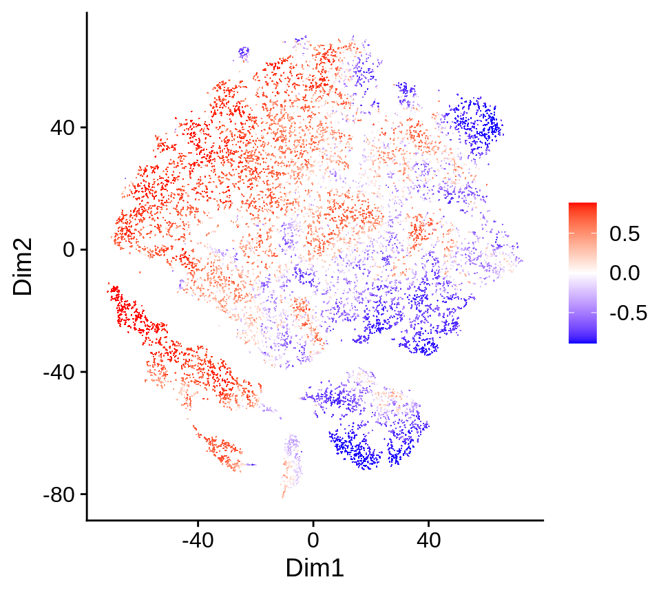
The prediction values are overlayed on the 2D embedding in the pred.plot slot of the output.
da_cells$pred.plot
DAseq runs a random permutation on the labels to generate the null distribution for DA measure. We can check the permutation results in the rand.plot slot.
da_cells$rand.plot
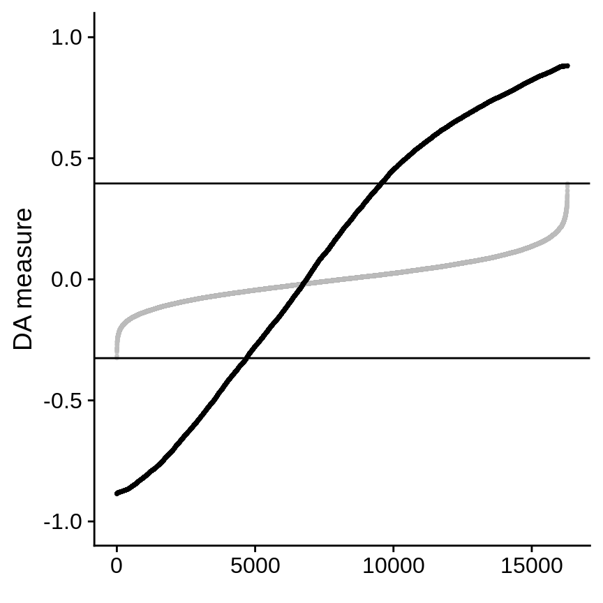
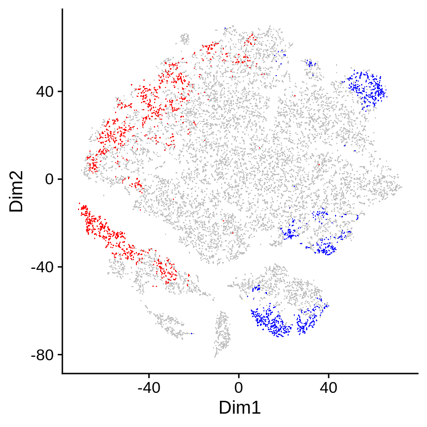
By default, cells with DA measure values larger than the maximum or small than the minumum than permutated DA measure are selected as DA cells. The threshold can be changed by running updateDAcells() to look at the most salient DA cells. In this data, we use 0.8 (for non-responder) and -0.8 (for responder).
da_cells <- updateDAcells(
  X = da_cells, pred.thres = c(-0.8,0.8),
  plot.embedding = X.2d.melanoma
)
Selected DA cells are highlighted in the 2D embedding in the da.cells.plot slot. Cells in red are in the top (these cells are more abundant in non-responder samples), blue in the bottom (these cells are more abundant in responder samples).
da_cells$da.cells.plot
Get DA regions
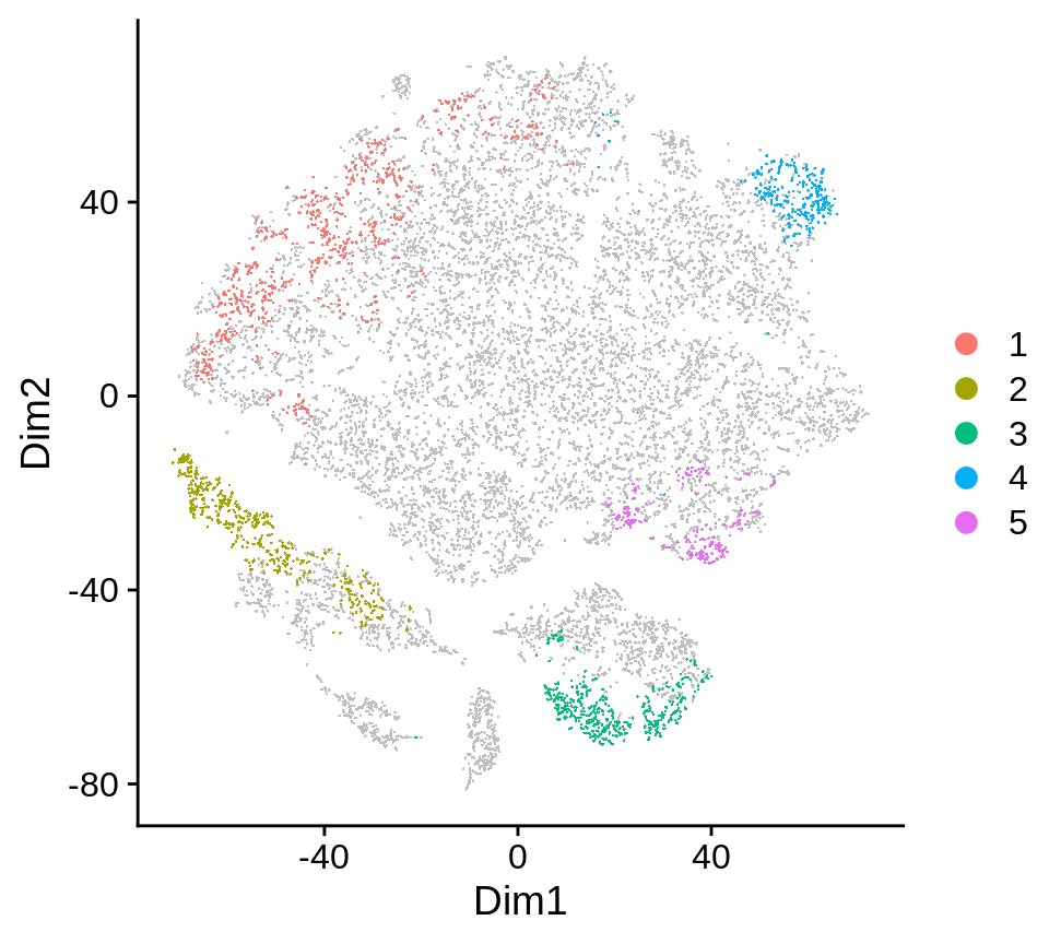
In this step, selected DA cells will be clustered into several coherent regions, which represent the DA cell subpopulations. Several input parameters are identical to that of getDAcells(): X, cell.labels, labels.1, labels.2, plot.embedding.
Other input includes:
-
da.cells: the output ofgetDAcells() -
resolution: clustering parameter, default 0.05, use a larger value to group DA cells into more regions -
min.cell: minimum number of cells, regions with fewer cells will be removed, default is to use the minumum k value in thek.vector
da_regions <- getDAregion(
  X = X.melanoma,
  da.cells = da_cells,
  cell.labels = X.label.melanoma,
  labels.1 = labels_res,
  labels.2 = labels_nonres,
  resolution = 0.01,
  plot.embedding = X.2d.melanoma,
)
The output is a list of results:
-
da.region.label, DA subpopulation labels for all the cells, 0 means non-DA cells -
DA.stat, statistics of each DA subpopulation
str(da_regions[1:2])
## List of 2
##  $ da.region.label: num [1:16291] 0 0 0 0 0 0 0 0 0 0 ...
##  $ DA.stat        : num [1:5, 1:3] 0.973 0.965 -0.933 -0.976 -0.904 ...
##   ..- attr(*, "dimnames")=List of 2
##   .. ..$ : NULL
##   .. ..$ : chr [1:3] "DA.score" "pval.wilcoxon" "pval.ttest"
Clustering result is shown in the plot: da.region.plot slot.
da_regions$da.region.plot
Get markers for each DA subpopulation with STG
The final step of DAseq is to characterize each DA subpopulation by detecting genes that seprate the DA subpopulation from the rest of the cells through STG (stochastic gates).
The gene expression data is NOT included in the DAseq package and needs to be downloaded. This code will download the data to the current working directory, and load this data into R.
download.file(
  "ftp://ftp.ncbi.nlm.nih.gov/geo/series/GSE120nnn/GSE120575/suppl/GSE120575_Sade_Feldman_melanoma_single_cells_TPM_GEO.txt.gz",
  "./GSE120575_Sade_Feldman_melanoma_single_cells_TPM_GEO.txt.gz"
)
X.data.melanoma <- read.table(
  "./GSE120575_Sade_Feldman_melanoma_single_cells_TPM_GEO.txt.gz",
  sep = "\t", header = F, row.names = 1, stringsAsFactors = F, skip = 2
)
X.data.melanoma <- as.matrix(X.data.melanoma[,-16292])
Then, we will use STG to identify markers for each DA subpopulation. The input parameters for STG are the normalized gene expression matrix, and the output from the function getDAregion().
STG_markers <- STGmarkerFinder(
  X = X.data.melanoma,
  da.regions = da_regions,
  lambda = 1.5, n.runs = 5, return.model = T,
  python.use = python2use, GPU = GPU
)
The output is a list of results:
-
da.markers, a list of data frames, each data frame contains markers for each DA subpopulation -
accuracy, accuracy of STG for each DA subpopulation -
model, the actual model from STG for each DA subpopulation, please refer to the documentation ofSTGmarkerFinder()
Top markers for DA region 5 are shown:
head(STG_markers$da.markers[["5"]])
##        gene avg_logFC       p_value
## TCF7   TCF7 1.8865021 4.261047e-122
## RPL13 RPL13 0.1765772 2.421585e-113
## RPL3   RPL3 0.2037486 1.516596e-102
## LEF1   LEF1 2.3623672 6.638429e-102
## RPS6   RPS6 0.2002730 2.013261e-100
## RPS3A RPS3A 0.2040410  2.452806e-98
In the model slot, predictions from STG are available. These predictions are linear combinations of a limited set of genes that best separate the DA subpopulation from the rest of the cells.
For example, here we will plot the prediction value from STG for DA subpopulation 5: the pred slot of the 5th list in the model slot of the output.
plotCellScore(
  X = X.2d.melanoma, score = STG_markers$model[["5"]]$pred
)
